An Unhinged Introduction to State Space Models: Act 2

Bayes

Stan

Stan takes the stage: parameter inference, posterior interrogation, and answering the question that started it all

Published

January 1, 2026

Code

library(kableExtra)
library(tidyverse)

# rstudioapi::getActiveDocumentContext()$path |> dirname() |> setwd()

state_space_utils <- new.env()
source('state_space_model_utilities.R', state_space_utils)

# Reproduce the same data from Part 1
set.seed(1234)
season_length <- 7; number_seasons <- 10
n_tot <- season_length * number_seasons
x1 <- (cumsum(rnorm(n_tot, 0,0.5)) + rnorm(n_tot, 0,.01)) |> abs()
x2 <- (cumsum(rnorm(n_tot, 0,0.5)) + rnorm(n_tot, 0,.01)) |> abs()
x_mat <- cbind(x1,x2)
beta_vec <- c(-1,1)

ss <- cos(seq(0,2*pi, length.out=season_length))*1
ss <- ss - mean(ss)
ss_vec <- c(ss)[-length(ss)]
ss_var <- 0.01^2;

slope_start <- 0; slope_var <- 1e-30; slope_vec <- c(slope_start)

mu_start <- rnorm(1,0,1); mu_var <- 0.05^2; mu_vec <- c(mu_start)

noise_var <- 0.5

y_vec <- ss_comp <-  c()
for (i in 1:n_tot){
  ss_comp <- c(ss_vec[1], ss_comp)
  y_vec <- c(y_vec, mu_vec[i] + (x_mat %*% beta_vec)[i] + ss_vec[1] + rnorm(1,0,sqrt(noise_var)))
  ss_vec <- c(-sum(ss_vec) + rnorm(1, 0, sqrt(ss_var)), ss_vec[-length(ss_vec)])
  slope_vec <- c(slope_vec, slope_vec[i] + rnorm(1, 0, sqrt(slope_var)))
  mu_vec <- c(mu_vec, mu_vec[i] + slope_vec[i] + rnorm(1, 0,sqrt(mu_var)))
}

is_new_prod_live <- seq_along(y_vec) >= length(y_vec) - 9
y_vec[is_new_prod_live] <- abs(y_vec[is_new_prod_live])*0.5 +
  y_vec[is_new_prod_live]

y_vec_no_prod <- y_vec[!is_new_prod_live]

Previously, on LENI Drinkware

Welcome back. If you missed Act 1, here’s the short version: LENI launched Tumbler v2™, sales went up, and we want to know how much of that increase is actually from the new product versus just industry trends, seasonality, and good vibes from our competitors “Abominable Snowman” and “Bigfoot”. We introduced the state space framework:

\[y_t = Z_t\alpha_t + \varepsilon_t\] \[\alpha_{t+1} = T_t \alpha_t + R_t \eta_t\]

We learned how to filter (forward pass), smooth (backward pass), and simulate draws from $P(\alpha|Y_n)$ using the Durbin and Koopman trick (Durbin and Koopman 2002). The ensemble has been cast, the understudies have rehearsed, the stage is set.

But here’s the thing: in Act 1, we knew the variance parameters. We hand-delivered $H_t$, $Q_t$, and $P_1$ to the Kalman filter like a stage manager distributing scripts. In the real world, nobody hands you these. You have to figure them out. This is where Stan enters stage left.

Enter Stan, Stage Left

The Director’s Vision

Stan is a probabilistic programming language built for Bayesian inference. It allows us to define our model in terms of priors, likelihoods, and generative structure without having to worry about specific maximum likelihood algorithms. We just let Stan turn the Bayesian crank to perform inference.

For our purposes, Stan will serve as the director of this production. It’s going to look at the raw time series, figure out the variance parameters that best explain the data, and simultaneously generate full posterior draws of the latent state $\alpha_t$.

The beautiful thing about the state space formulation is that the Kalman filter gives us a decomposition of the likelihood for free. You don’t need to write out some nightmarish joint density over all the latent states. Instead, you get what’s called the prediction error decomposition:

\[\log p(Y_n | \theta) = -\frac{n}{2}\log 2\pi - \frac{1}{2}\sum_{t=1}^n\left[\log F_t + v_t^2 F_t^{-1}\right]\]

where $v_t = y_t - Z_t a_t$ is the one-step-ahead prediction error and $F_t = \text{Var}(v_t|Y_{t-1})$ is its variance. Both of these fall directly out of the Kalman filter recursions. This is the same $v_t$ and $F_t$ you met in Act 1. They were side characters then, but now they’re the stars.

The Trick

Here’s the punchline. If $v_t | Y_{t-1} \sim \mathcal{N}(0, F_t)$, then we can write the Stan model block as:

model {
  var_vec ~ exponential(1);
  P_1_diag ~ exponential(1);
  noise_var ~ exponential(1);

  v ~ normal(mu_placeholder, F);
}

That’s it. That’s the likelihood. The vector v and F are computed deterministically in transformed parameters via the Kalman filter, and Stan’s sampler does the rest. The mu_placeholder is just a vector of zeros (since $\mathbb{E}[v_t|Y_{t-1}] = 0$ by construction). The parameter F here is actually $\sqrt{F_t}$ since Stan’s normal parameterization takes the standard deviation, not the variance.

This is incredibly elegant. Stan only needs to explore a tiny parameter space (the variance components), while the Kalman filter handles all the latent state bookkeeping deterministically. No marginalization tricks, no augmented state vectors in the sampler. Just a handful of variance parameters and a very efficient filter.

The Script

Full Stan Program

Let’s walk through the full Stan program piece by piece. The complete file is structured as:

functions {
  #include state_space_functions.stan
}
data { ... }
transformed data { ... }
parameters { ... }
transformed parameters { ... }
model { ... }
generated quantities { ... }

The #include directive pulls in all of our matrix construction and Kalman filter machinery. Let’s start with what Stan needs from us.

The Data Block

data {
  int<lower=1> N;
  vector[N] y;
  int<lower=0, upper=1> has_slope;
  int<lower=0> n_covar;
  int<lower=0> n_seasons;
  matrix[N,n_covar] X_mat;
}

Nothing surprising here. We pass in our time series y, the covariate matrix X_mat (columns for Abominable Snowman and Bigfoot), and a set of flags that configure the model structure. The has_slope toggle lets us include or exclude a linear trend component. For our LENI analysis we set has_slope=0 since the competitor covariates should absorb any industry-level drift.

Transformed Data: Building the System Matrices

transformed data{
  int season_cont = n_seasons > 2 ? n_seasons - 1 : 0;
  int a_size = has_slope + n_covar + season_cont + 1;
  int has_season =  n_seasons > 2 ? 1 : 0;
  int has_regress = n_covar > 0 ? 1 : 0;

  array[N] row_vector[a_size] Z_arr = gen_z_arr(N, has_slope, X_mat, n_seasons);
  matrix[a_size, a_size] T_mat = gen_T_mat(has_slope, n_covar, n_seasons);
  matrix[a_size, 1 + has_slope + has_season] R_mat = gen_R_mat(has_slope, n_covar, n_seasons);
}

This is where the model configuration crystallizes into concrete matrices. The three generator functions (gen_z_arr, gen_T_mat, gen_R_mat) build our entire system of equations based on the toggle flags. Let’s look at each one.

The Design Matrix: `gen_z_arr`

Recall that $Z_t$ maps from the latent state $\alpha_t$ down to the observation $y_t$. For our LENI model with 7-day seasonality and 2 covariates:

\[Z_t = \begin{bmatrix} 1 & 1 & 0 & 0 & 0 & 0 & 0 & x_{a,t} & x_{b,t}\end{bmatrix}\]

The leading 1 selects the trend $\mu_t$. The second 1 selects the current seasonal effect $\tau_t$. The zeros skip the $s-2$ carried-over seasonal states. The trailing entries are the covariate values at time $t$. Here’s how the Stan function builds this:

array[] row_vector gen_z_arr(int n, int include_slope, matrix x_mat, int n_seasons){
  int season_cont = n_seasons > 2 ? n_seasons - 1 : 0;
  int z_size = include_slope + cols(x_mat) + season_cont + 1;
  array[n] row_vector[z_size] z_arr;

  row_vector[1 + season_cont + include_slope] left_pad;

  if (n_seasons > 2){
    left_pad = append_col(
      1,
      append_col(
        rep_row_vector(0, include_slope),
        append_col(1, rep_row_vector(0, n_seasons - 2))
      )
    );
  }
  else {
    left_pad = append_col(1, rep_row_vector(0, include_slope));
  }

  if (cols(x_mat) > 0){
    for (i in 1:n)
      z_arr[i] = append_col(left_pad, x_mat[i]);
  }
  else{
    for (i in 1:n)
      z_arr[i] = left_pad;
  }
  return z_arr;
}

The left_pad is the static portion (trend + season selectors). We then append the time-varying covariate row for each observation. This is the only matrix that changes with $t$, because $x_{a,t}$ and $x_{b,t}$ are different at every time step.

The Transition Matrix: `gen_T_mat`

$T_t$ evolves the state forward. For our model it looks like:

Generate T matrix

T_mat <- state_space_utils$gen_T_mat(include_slope=F, n_regress=2, n_seasons=7)
rownames(T_mat) <- colnames(T_mat) <- c('mu', paste0('tau_',0:5), 'beta_a', 'beta_b')
T_mat |> kable() |> kable_styling(position='center', full_width=F) |>
  column_spec(1, bold=T)

	mu	tau_0	tau_1	tau_2	tau_3	tau_4	tau_5	beta_a	beta_b
mu	1	0	0	0	0	0	0	0	0
tau_0	0	-1	-1	-1	-1	-1	-1	0	0
tau_1	0	1	0	0	0	0	0	0	0
tau_2	0	0	1	0	0	0	0	0	0
tau_3	0	0	0	1	0	0	0	0	0
tau_4	0	0	0	0	1	0	0	0	0
tau_5	0	0	0	0	0	1	0	0	0
beta_a	0	0	0	0	0	0	0	1	0
beta_b	0	0	0	0	0	0	0	0	1

The structure encodes our modeling assumptions:

Row 1: $\mu_{t+1} = \mu_t$ (random walk, disturbance added later)
Rows 2-7: The seasonal shift register. Row 2 computes $\tau_{t+1} = -\sum_{j=1}^{s-1}\tau_{t+1-j}$. Rows 3-7 shift the seasonal history down by one slot.
Rows 8-9: $\beta_a$ and $\beta_b$ persist unchanged (identity block)

The Stan function gen_T_mat builds this programmatically. The seasonal block is the trickiest part: it places $-1$s across the top row of the seasonal sub-matrix and a sub-diagonal of $1$s to shift history.

The Selection Matrix: `gen_R_mat`

$R_t$ decides which elements of $\alpha_t$ receive stochastic shocks. For LENI:

Generate R matrix

R_mat <- state_space_utils$gen_R_mat(include_slope=F, n_regress=2, n_seasons=7)
rownames(R_mat) <- c('mu', paste0('tau_',0:5), 'beta_a', 'beta_b')
colnames(R_mat) <- c('eta_mu', 'eta_tau')
R_mat |> kable() |> kable_styling(position='center', full_width=F) |>
  column_spec(1, bold=T)

	eta_mu	eta_tau
mu	1	0
tau_0	0	1
tau_1	0	0
tau_2	0	0
tau_3	0	0
tau_4	0	0
tau_5	0	0
beta_a	0	0
beta_b	0	0

Only $\mu_t$ and $\tau_t$ receive disturbances. The carried seasonal states and regression coefficients get nothing. This is how we encode “regression coefficients are static over time” without any special machinery. We simply don’t disturb them.

Parameters: What Stan Explores

parameters{
  vector<lower=0>[cols(R_mat)] var_vec;
  vector<lower=0>[a_size] P_1_diag;
  real<lower=0> noise_var;
}

The entire parameter space consists of:

var_vec: the diagonal of $Q_t$. For our model, this is $[\sigma^2_\mu, \sigma^2_\tau]$. Two parameters.
P_1_diag: the diagonal of the initial state covariance $P_1$. Nine parameters (one per element of $\alpha_1$).
noise_var: the observation noise $H_t = \sigma^2_y$. One parameter.

That’s twelve total parameters for Stan to explore. Everything else (the full latent state trajectory, the filtered/smoothed estimates, the prediction errors) is computed deterministically by the Kalman filter. This is a remarkably efficient use of HMC’s time.

Transformed Parameters: The Kalman Filter Lives Here

transformed parameters{
  vector[a_size * N + (2 * N)] k_obj = kalman_filter_smooth(
    N, y, rep_vector(0, a_size), P_1_diag,
    noise_var, var_vec, T_mat, R_mat, Z_arr
  );
  vector[N] F = sqrt(get_F(k_obj, s));
  vector[N] v = get_v(k_obj, s);
}

Every time Stan proposes a new set of variance parameters, the Kalman filter runs to completion and produces $v_t$ and $F_t$ for all $t$. These get fed directly into the likelihood. The k_obj is a packed vector containing the smoothed states, $F$, and $v$. We pack it this way because Stan functions can only return a single object. Not pretty, but functional.

The packing/unpacking is handled by helper functions:

vector get_F(vector kalman_object, array[] int s){
  return segment(kalman_object, 1 + s[1], s[2]);
}

vector get_v(vector kalman_object, array[] int s){
  return segment(kalman_object, 1 + sum(s[1:2]), s[3]);
}

The array s stores the segment boundaries so we can slice correctly. It’s the Stan equivalent of a ragged array, implemented via flat vectors and index arithmetic.

Generated Quantities: Simulation

generated quantities{
  array[N] vector[a_size] alpha_sim = simulate_state_rng(
    k_obj, N, s, s_evolve, y, rep_vector(0,a_size), P_1_diag,
    noise_var, var_vec, T_mat, R_mat, Z_arr
  );
  array[1 + has_season + has_regress] vector[N] trend_comp =
    extract_trends(alpha_sim, N, Z_arr, has_slope, n_covar, n_seasons);
}

This is the Durbin and Koopman simulation smoother from Act 1, now running inside Stan’s sampler. At every MCMC iteration (after the warmup), it:

Draws $\alpha_1^+$ from $\mathcal{N}(0, P_1)$
Evolves the system forward to produce $\alpha^+$ and $y^+$
Smooths the synthetic series to get $\hat{\alpha}^+$
Computes $\tilde{\alpha} = \alpha^+ - \hat{\alpha}^+ + \hat{\alpha}$

The result is a draw from the posterior $P(\alpha | Y_n, \theta)$ conditional on that iteration’s parameter values. Across all post-warmup iterations, you get a full posterior distribution over every latent state at every time point. Then extract_trends decomposes each draw into its constituent components: trend, seasonal, and regression.

The Kalman Filter Implementation

Let me walk through the core filtering and smoothing function since it’s doing all the heavy lifting. I’ll annotate the key sections:

vector kalman_filter_smooth(int n, vector y, vector a_1, vector P_1_diag,
                            real noise_var, vector var_vec, matrix T_mat,
                            matrix R_mat, array[] row_vector Z_arr){
  matrix[size(P_1_diag), size(P_1_diag)] P_1 = diag_matrix(P_1_diag);

  // === FORWARD PASS ===
  vector[n] F;
  vector[n] v;
  array[n+1] vector[num_elements(a_1)] a;
  a[1] = a_1;

  array[n+1] matrix[rows(P_1), cols(P_1)] P;
  P[1] = P_1;

  array[n] vector[num_elements(a_1)] K;
  array[n] matrix[rows(T_mat), cols(T_mat)] L;
  matrix[num_elements(var_vec), num_elements(var_vec)] Q_mat = diag_matrix(var_vec);

  for (i in 1:n){
    // Prediction error and its variance
    v[i] = y[i] - dot_product(Z_arr[i], a[i]);
    F[i] = Z_arr[i] * P[i] * Z_arr[i]' + noise_var;

    // Kalman gain
    K[i] = T_mat * P[i] * Z_arr[i]' * (1 / F[i]);
    L[i] = T_mat - K[i] * Z_arr[i];

    // State prediction
    P[i + 1] = T_mat * P[i] * L[i]' + R_mat * Q_mat * R_mat';
    a[i + 1] = (T_mat * a[i]) + (K[i] * v[i]);
  }

  // === BACKWARD PASS ===
  array[n + 1] vector[num_elements(a_1)] r =
    rep_array(rep_vector(0, num_elements(a_1)), n + 1);
  array[n] vector[num_elements(a_1)] alpha_smooth;

  for (d in 1:n){
    int i = n - d + 1;  // Reverse: n, n-1, ..., 1
    r[i] = Z_arr[i]' * (1/F[i]) * v[i] + L[i]' * r[i + 1];
    alpha_smooth[i] = a[i] + P[i] * r[i];
  }

  // Pack everything into a single vector and return
  ...
}

The forward pass is a direct translation of the Kalman filter equations from Act 1. The backward pass implements the smoothing recursion $r_{t-1} = Z_t^\prime F_t^{-1} v_t + L_t^\prime r_t$ with $\hat{\alpha}_t = a_t + P_t r_{t-1}$. Notice that r is initialized at zero for r[n+1] (corresponding to $r_n = 0$) and the loop proceeds backwards.

One implementation detail worth noting: since $y_t$ is univariate, $F_t$ is a scalar and we can use 1/F[i] instead of a matrix inverse. This would need to change for a multivariate observation model.

Opening Night

Fitting the Model

With the script written and the cast assembled, it’s time for the performance. We fit the model using cmdstanr:

library(cmdstanr)
options(mc.cores = parallel::detectCores())

mod <- cmdstan_model('state_space.stan')

data <- list(
  N = length(y_vec_no_prod),
  y = y_vec_no_prod,
  has_slope = 0,
  n_seasons = 7,
  n_covar = 2,
  X_mat = cbind(x1, x2)[!is_new_prod_live, ]
)

fit <- mod$sample(
  data = data,
  chains = 4,
  parallel_chains = 4,
  iter_warmup = 200,
  iter_sampling = 200
)

We fit on y_vec_no_prod, the series excluding the post-launch observations. This is crucial. We’re training the model on the world before Tumbler v2™ existed, so that when we project forward, the model has no knowledge of the intervention.

Checking the Reviews

Before we trust any results, we need to make sure the sampler actually converged. The usual suspects:

fit$summary(variables = c('var_vec', 'noise_var', 'P_1_diag')) |> as.data.frame() |> 
  select(variable, mean, q5, q95, rhat, ess_bulk, ess_tail) |> 
  mutate(across(where(is.numeric), round, digits = 2)) |> head(7)

     variable mean   q5  q95 rhat ess_bulk ess_tail
1  var_vec[1] 0.04 0.00 0.14 1.01   551.99   549.72
2  var_vec[2] 0.03 0.00 0.10 1.00   938.26   477.82
3   noise_var 0.45 0.28 0.68 1.00   714.33   456.02
4 P_1_diag[1] 1.13 0.18 2.89 1.01   660.06   338.39
5 P_1_diag[2] 1.42 0.34 3.48 1.01   859.92   584.50
6 P_1_diag[3] 0.80 0.02 2.66 1.00   677.02   360.15
7 P_1_diag[4] 1.10 0.20 2.61 1.00   912.88   516.39

What we’re looking for:

$\hat{R} < 1.01$ for all parameters (chains mixed well)
ESS > 400 (enough effective samples)
No divergent transitions (geometry wasn’t pathological)

Since we generated this data ourselves, we have the luxury of checking parameter recovery. The true data generating process used:

Parameter	True Value
$\sigma^2_\mu$	$0.05^2 = 0.0025$
$\sigma^2_\tau$	$0.01^2 = 0.0001$
$\sigma^2_y$ (noise)	$0.5$

If the posterior intervals for var_vec[1], var_vec[2], and noise_var contain these values, the machinery is working correctly.

Recovering the Regression Coefficients

One of the most satisfying checks: do we recover the true $\beta$ values? Remember, the DGP used $\beta_a = -1$ and $\beta_b = 1$. These live in the last two elements of $\alpha_t$, and since we gave them no disturbance (via $R_t$), they should be approximately constant across time. We can inspect them at the final time step:

# Beta coefficients are in alpha_sim[N, 8] and alpha_sim[N, 9]
fit$summary(variables = c(
  sprintf('alpha_sim[%d,8]', length(y_vec_no_prod)),
  sprintf('alpha_sim[%d,9]', length(y_vec_no_prod))
))

# A tibble: 2 × 10
  variable       mean median     sd    mad     q5    q95  rhat ess_bulk ess_tail
  <chr>         <dbl>  <dbl>  <dbl>  <dbl>  <dbl>  <dbl> <dbl>    <dbl>    <dbl>
1 alpha_sim[6… -0.935 -0.939 0.0955 0.0812 -1.08  -0.764  1.00     653.     461.
2 alpha_sim[6…  0.800  0.798 0.141  0.135   0.574  1.04   1.01     709.     652.

If the model is working, we should see the posteriors for $\beta_a$ and $\beta_b$ centered near $-1$ and $1$ respectively.

Decomposing the Performance

Extracting the Components

The extract_trends function in generated quantities gives us three component arrays:

trend_comp[1,]: the underlying trend $\mu_t$
trend_comp[2,]: the seasonal component $\tau_t$
trend_comp[3,]: the regression component $\beta_a x_{a,t} + \beta_b x_{b,t}$

These components are additive. At any time $t$:

\[\hat{y}_t = \mu_t + \tau_t + \beta_a x_{a,t} + \beta_b x_{b,t}\]

Code

library(tidyverse)

# --- Color palette (dark blue anchored) ---
pal <- list(
  navy      = '#1B2838',
  blue      = '#2C5F8A',
  slate     = '#4A7FB5',
  copper    = '#C47E3F',
  sage      = '#5B8C6F',
  light_bg  = '#F7F9FC',
  grid      = '#D6DFE8'
)

# Extract posterior means for each component
t_comp <- fit$draws('trend_comp', format='df')
trend_mean <-  t_comp %>% select(starts_with('trend_comp[1,')) %>% colMeans()
season_mean <- t_comp %>% select(starts_with('trend_comp[2,')) %>% colMeans()
regress_mean <- t_comp %>% select(starts_with('trend_comp[3,')) %>% colMeans()

par(mfrow=c(4,1), mar=c(3,4.5,2.5,1),  family='sans')

# Panel 1: Observed
plot(y_vec_no_prod, type='b', pch=16, cex=0.8, lwd=1.5, col=pal$navy,
     main='', xlab='', ylab='',
     axes=FALSE, panel.first=grid(col=pal$grid, lty=1, lwd=0.5))
title(main='Observed Series', font.main=2, cex.main=1.3, col.main=pal$navy)
axis(1, lwd=2, col=pal$navy, col.axis=pal$navy, font=2)
axis(2, lwd=2, col=pal$navy, col.axis=pal$navy, font=2)
box(lwd=2, col=pal$navy)

# Panel 2: Trend
plot(trend_mean, type='l', lwd=3, col=pal$blue,
     main='', xlab='', ylab='',
     axes=FALSE, panel.first=grid(col=pal$grid, lty=1, lwd=0.5))
title(main=expression(bold(paste('Trend (', mu[t], ')'))), cex.main=1.3, col.main=pal$navy)
axis(1, lwd=2, col=pal$navy, col.axis=pal$navy, font=2)
axis(2, lwd=2, col=pal$navy, col.axis=pal$navy, font=2)
box(lwd=2, col=pal$navy)

# Panel 3: Seasonal
plot(season_mean, type='l', lwd=3, col=pal$sage,
     main='', xlab='', ylab='',
     axes=FALSE, panel.first=grid(col=pal$grid, lty=1, lwd=0.5))
title(main=expression(bold(paste('Seasonal (', tau[t], ')'))), cex.main=1.3, col.main=pal$navy)
axis(1, lwd=2, col=pal$navy, col.axis=pal$navy, font=2)
axis(2, lwd=2, col=pal$navy, col.axis=pal$navy, font=2)
box(lwd=2, col=pal$navy)

# Panel 4: Regression
plot(regress_mean, type='l', lwd=3, col=pal$copper,
     main='', xlab='', ylab='',
     axes=FALSE, panel.first=grid(col=pal$grid, lty=1, lwd=0.5))
title(main=expression(bold(paste('Regression (', beta %.% x, ')'))), cex.main=1.3, col.main=pal$navy)
axis(1, lwd=2, col=pal$navy, col.axis=pal$navy, font=2)
axis(2, lwd=2, col=pal$navy, col.axis=pal$navy, font=2)
box(lwd=2, col=pal$navy)

This decomposition is one of the primary selling points of the state space approach. You don’t just get a fitted line. You get a full accounting of where the signal comes from at every point in time.

The Moment of Truth

Counterfactual Prediction

Here’s the scene we’ve been building towards. We’ve trained our model on the pre-launch era. The model has learned:

The underlying trend dynamics ($\sigma^2_\mu$)
The seasonal rhythm ($\sigma^2_\tau$, and the seasonal state history)
How LENI’s sales relate to the broader drinkware industry ($\beta_a$, $\beta_b$)
The observation noise ($\sigma^2_y$)

Now we ask: what would LENI’s sales have looked like in the 10 post-launch periods if Tumbler v2™ had never been released?

The procedure:

Take the posterior draws of all parameters from the fitted model
For each draw, use the final smoothed state $\hat{\alpha}_n$ as the launching point
Evolve the system forward for 10 time steps using equations (1) and (2), plugging in the actual competitor covariate values from the post-launch period
The resulting $\hat{y}_{n+1}, \dots, \hat{y}_{n+10}$ is our counterfactual: what the model predicts without any intervention

# Extract posterior draws of the final smoothed state and parameters
n_pre <- length(y_vec_no_prod)
n_post <- sum(is_new_prod_live)  # 10 periods
x_post <- cbind(x1, x2)[is_new_prod_live, ]

# For each posterior draw, roll forward
n_draws <- 800
counterfactual <- matrix(NA, nrow = n_draws, ncol = n_post)

draws <- fit$draws(format = 'draws_matrix')

for (d in 1:n_draws) {
  # Get the final alpha state for this draw
  alpha_n <- draws[d, sprintf('alpha_sim[%d,%d]', n_pre, 1:9)]
  var_d <- draws[d, c('var_vec[1]', 'var_vec[2]')]
  noise_d <- draws[d, 'noise_var']

  # Build Z for post-launch period (same structure, new x values)
  alpha_curr <- as.numeric(alpha_n)

  for (t in 1:n_post) {
    z_t <- c(1, 1, rep(0, 5), x_post[t, ])
    # Expected observation (no noise for point prediction)
    counterfactual[d, t] <- sum(z_t * alpha_curr)

    # Evolve state forward
    alpha_curr <- as.numeric(T_mat %*% alpha_curr) +
      as.numeric(R_mat %*% rnorm(2, 0, sqrt(as.numeric(var_d))))
  }
}

Quantifying the Incremental

The incremental effect of Tumbler v2™ at each post-launch time point is simply:

\[\Delta_t = y_t^{\text{actual}} - \hat{y}_t^{\text{counterfactual}}\]

Since we have a full posterior distribution over $\hat{y}_t^{\text{counterfactual}}$, we get a full posterior distribution over $\Delta_t$. This means we can make probabilistic statements like “there is a 95% probability that the incremental sales from Tumbler v2™ are between $X and $Y.”

Code

y_actual_post <- y_vec[is_new_prod_live]

# --- Color palette (dark blue anchored) ---
pal <- list(
  navy      = '#1B2838',
  blue      = '#2C5F8A',
  slate     = '#4A7FB5',
  copper    = '#C47E3F',
  sage      = '#5B8C6F',
  light_bg  = '#F7F9FC',
  grid      = '#D6DFE8'
)

# Compute incremental for each draw
incremental <- sweep(-counterfactual, 2, y_actual_post, '+')

# Posterior summaries
inc_mean <- colMeans(incremental)
inc_q05 <- apply(incremental, 2, quantile, 0.05)
inc_q95 <- apply(incremental, 2, quantile, 0.95)

# Total incremental
total_inc <- rowSums(incremental)
cat(sprintf("Posterior mean total incremental: $%.2f\n", mean(total_inc)))

Posterior mean total incremental: $36.77

Code

cat(sprintf("95%% credible interval: [$%.2f, $%.2f]\n",
            quantile(total_inc, 0.025), quantile(total_inc, 0.975)))

95% credible interval: [$27.14, $47.01]

Code

# Plot
par(mar=c(4.5, 5, 3, 1), family='sans')
x_idx <- (n_pre + 1):(n_pre + n_post)

plot(seq_along(y_vec), y_vec, type='b', pch=16, cex=0.8, lwd=1.5,
     main='', xlab='', ylab='',
     col=ifelse(is_new_prod_live, pal$copper, pal$navy),
     axes=FALSE, panel.first=grid(col=pal$grid, lty=1, lwd=0.5))
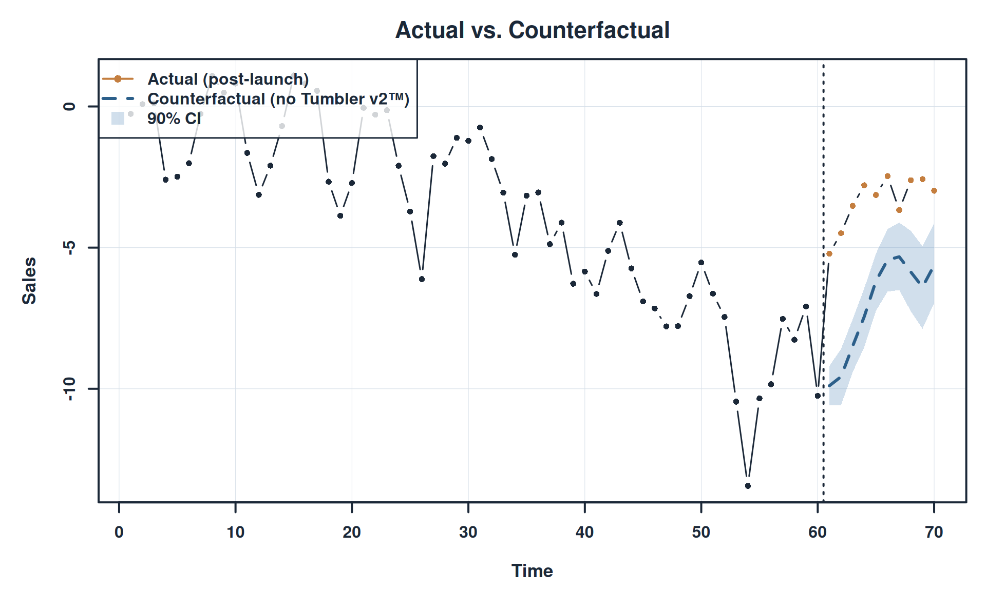
title(main='Actual vs. Counterfactual', font.main=2, cex.main=1.4, col.main=pal$navy)
title(xlab='Time', ylab='Sales', font.lab=2, cex.lab=1.1, col.lab=pal$navy)
axis(1, lwd=2, col=pal$navy, col.axis=pal$navy, font=2)
axis(2, lwd=2, col=pal$navy, col.axis=pal$navy, font=2)

# Counterfactual with uncertainty
cf_mean <- colMeans(counterfactual)
cf_q05 <- apply(counterfactual, 2, quantile, 0.05)
cf_q95 <- apply(counterfactual, 2, quantile, 0.95)

polygon(c(x_idx, rev(x_idx)), c(cf_q05, rev(cf_q95)),
        col=adjustcolor(pal$slate, 0.25), border=NA)
lines(x_idx, cf_mean, lwd=3, col=pal$blue, lty=2)

abline(v = n_pre + 0.5, lwd=2, lty=3, col=pal$navy)
legend('topleft',
       legend=c('Actual (post-launch)', 'Counterfactual (no Tumbler v2\u2122)', '90% CI'),
       col=c(pal$copper, pal$blue, NA), lwd=c(2,3,NA), lty=c(1,2,NA),
       pch=c(16, NA, 22), pt.bg=c(NA, NA, adjustcolor(pal$slate, 0.25)),
       pt.cex=c(1, 1, 2), text.font=2, text.col=pal$navy,
       bg=adjustcolor('white', 0.8), box.lwd=1.5, box.col=pal$navy)
box(lwd=2, col=pal$navy)

The gap between the copper points (actual post-launch sales) and the blue dashed line (counterfactual) is the incremental effect of Tumbler v2™. The shaded region shows our uncertainty about the counterfactual. Where the copper points lie above the shaded region, we can be quite confident that the uplift is real and not just noise.

The Cumulative Picture

For a final summary, we can look at the cumulative incremental sales over the post-launch window:

Code

# --- Color palette (dark blue anchored) ---
pal <- list(
  navy      = '#1B2838',
  blue      = '#2C5F8A',
  slate     = '#4A7FB5',
  copper    = '#C47E3F',
  sage      = '#5B8C6F',
  light_bg  = '#F7F9FC',
  grid      = '#D6DFE8'
)

cum_inc <- t(apply(incremental, 1, cumsum))
cum_mean <- colMeans(cum_inc)
cum_q05 <- apply(cum_inc, 2, quantile, 0.05)
cum_q95 <- apply(cum_inc, 2, quantile, 0.95)

par(mar=c(4.5, 5, 3, 1), family='sans')

plot(1:n_post, cum_mean, type='l', lwd=3, col=pal$blue,
     main='', xlab='', ylab='',
     ylim=range(c(cum_q05, cum_q95)),
     axes=FALSE, panel.first=grid(col=pal$grid, lty=1, lwd=0.5))
title(main='Cumulative Incremental Sales from Tumbler v2\u2122',
      font.main=2, cex.main=1.4, col.main=pal$navy)
title(xlab='Days Since Launch', ylab='Cumulative $ Incremental',
      font.lab=2, cex.lab=1.1, col.lab=pal$navy)
axis(1, lwd=2, col=pal$navy, col.axis=pal$navy, font=2)
axis(2, lwd=2, col=pal$navy, col.axis=pal$navy, font=2)

polygon(c(1:n_post, n_post:1), c(cum_q05, rev(cum_q95)),
        col=adjustcolor(pal$slate, 0.2), border=NA)
abline(h=0, lty=2, lwd=2, col=pal$navy)
box(lwd=2, col=pal$navy)
legend('topleft', legend=c('Posterior Mean', '90% Credible Interval'),
       col=c(pal$blue, NA), lwd=c(3, NA), pch=c(NA, 22),
       pt.bg=c(NA, adjustcolor(pal$slate, 0.2)), pt.cex=c(1, 2),
       text.font=2, text.col=pal$navy,
       bg=adjustcolor('white', 0.8), box.lwd=1.5, box.col=pal$navy)

If the credible interval stays above zero, we have strong evidence that the launch generated real incremental revenue.

Curtain Call

What We Built

Let’s take stock. Across these two acts we:

Defined a flexible state space system that decomposes a time series into trend, seasonality, and regression components
Implemented the Kalman filter and smoother in Stan’s function language
Used the prediction error decomposition as a likelihood, letting Stan explore only the variance parameters while the filter handles the latent states
Generated full posterior draws of the latent state via the Durbin and Koopman simulation smoother
Projected the fitted model forward to build a counterfactual, then compared it against reality to quantify the incremental effect of Tumbler v2™

The total parameter count that Stan actually sampled was twelve. Twelve parameters to characterize an entire time series decomposition with full uncertainty quantification. The Kalman filter did the rest.

Limitations and Extensions

No model is perfect, and ours has some notable limitations:

Linearity: The observation equation $y_t = Z_t \alpha_t + \varepsilon_t$ is linear. If the true relationship between covariates and sales is nonlinear, this model will miss it. Extensions using the unscented Kalman filter or particle filters can handle nonlinear state transitions, but at significant computational cost.

Exogeneity: We assumed that Abominable Snowman and Bigfoot’s sales are exogenous to LENI’s. If Tumbler v2™ also affected competitor sales (say, cannibalizing their market share), then our counterfactual would be biased. A multivariate state space model with $p > 1$ could address this.

Prior sensitivity on $P_1$: The initial state covariance matters more than you’d think, especially for short series. With 60 pre-launch observations we have reasonable burn-in, but for very short series you might want to use the diffuse initialization approach from Chapter 5 of (Durbin and Koopman 2012).

Static coefficients: We assumed $\beta_a$ and $\beta_b$ are constant over time. If the relationship between LENI and its competitors is evolving (perhaps due to market dynamics), time-varying coefficients can be enabled simply by adding rows to $R_t$ and corresponding entries in $Q_t$.

Final Bow

State space models are old. The Kalman filter dates to 1960. But the combination of a classical, well-understood filtering framework with modern Bayesian inference via Stan gives us something genuinely powerful: principled uncertainty quantification over decomposed time series components, all from a handful of variance parameters and some clever linear algebra.

The audience applauds. The curtain falls. LENI’s stock price goes up.

References

Durbin, James, and Siem Jan Koopman. 2012. Time Series Analysis by State Space Methods. Oxford University Press. https://doi.org/10.1093/acprof:oso/9780199641178.001.0001.

Durbin, J., and S. J. Koopman. 2002. “A Simple and Efficient Simulation Smoother for State Space Time Series Analysis.” Biometrika 89 (3): 603–15. http://www.jstor.org/stable/4140605.

Parameter	True Value
\(\sigma^2_\mu\)	\(0.05^2 = 0.0025\)
\(\sigma^2_\tau\)	\(0.01^2 = 0.0001\)
\(\sigma^2_y\) (noise)	\(0.5\)

Previously, on LENI Drinkware

Enter Stan, Stage Left

The Director’s Vision

The Trick

The Script

Full Stan Program

The Data Block

Transformed Data: Building the System Matrices

The Design Matrix: gen_z_arr

The Transition Matrix: gen_T_mat

The Selection Matrix: gen_R_mat

Parameters: What Stan Explores

Transformed Parameters: The Kalman Filter Lives Here

Generated Quantities: Simulation

The Kalman Filter Implementation

Opening Night

Fitting the Model

Checking the Reviews

Recovering the Regression Coefficients

Decomposing the Performance

Extracting the Components

The Moment of Truth

Counterfactual Prediction

Quantifying the Incremental

The Cumulative Picture

Curtain Call

What We Built

Limitations and Extensions

Final Bow

References

The Design Matrix: `gen_z_arr`

The Transition Matrix: `gen_T_mat`

The Selection Matrix: `gen_R_mat`